Moving Horizon Estimation
Consider a state estimation problem using a Moving Horizon Estimator (MHE). The basic problem consists of finding the state estimate \(x_{mhe}\) over a horizon \(N\) the minimizes the sum of squares between the predicted measurements \((y[t] - Cx_{mhe}[t])\) and the true measurements as well as the the state estimate and the predicted state \((x_{mhe}[t+1] - (Ax_{mhe}[t]) + Bu[t])\) where \(A, B, C\) are the system matrices, \(y\) are the prior measurements (including the current), and \(u\) are the prior controls. The basic optimization problem is given by:
where \(\gamma\) is a weighing parameter that balances the relative importance of the prior model predictions.
The system dynamics, including the noise, are given by:
where \(\mathbf{w}, \mathbf{v}\) are the process and measurement noise.
In addition to the basic problem, we may know some information about the state, such as its bounds \(x_{min}, x_{max}\). Consider the following chance constraints on the state estimate that incorporate these bounds:
Assume that \(\mathbf{w}, \mathbf{v}\) follow Gaussian distributions with means \(\overline{w}, \overline{v}\) and variances \(\sigma_w^2, \sigma_v^2\): \(\mathbf{w} \sim \mathcal{N}(\overline{w}, \sigma^2_w)\), \(\mathbf{v} \sim \mathcal{N}(\overline{v}, \sigma^2_v)\).
The chance constraint can be reformulated into a deterministic constraint as follows:
where \(\Phi^{-1}\) is the inverse CDF of the standard normal Gaussian distribution. However, using cvxRiskOpt, these deterministic reformulation are not necessary and the chance constraint can be encoded directly into the CVXPY problem.
Example
In the following code, we solve the constrained moving horizon estimation problem with CVXPY and cvxRiskOpt.
import time
import cvxpy as cp
import numpy as np
import matplotlib.pyplot as plt
from scipy.stats import norm
from cvxRiskOpt.cclp_risk_opt import cclp_gauss

def dyn(x, u, w):
    return x + u + w

def meas(x, v):
    return x + v

sim_steps = 200
N_mhe = 10
w_mean, v_mean = 0, 0
w_var, v_var = 0.01, 10
u_min, u_max = -0.5, 0.5
x_min, x_max = 0, 60
x0 = 5  # initial state

x_mhe = cp.Variable(N_mhe + 1, 'x_mhe')
x_mhe0 = cp.Parameter(name='x_mhe0')
y_mhe = cp.Parameter(N_mhe + 1, 'y_mhe')
u_mhe = cp.Parameter(N_mhe, 'u_mhe')
mhe_obj = 0
constr = [x_mhe[0] == x_mhe0]
for t in range(N_mhe + 1):
    mhe_obj += cp.square(y_mhe[t] - meas(x_mhe[t], v_mean))
for t in range(N_mhe):
    mhe_obj += 100 * cp.square(x_mhe[t + 1] - dyn(x_mhe[t], u_mhe[t], w_mean))
    constr += [cclp_gauss(eps=0.05, a=-1, b=x_min,
                          xi1_hat=dyn(x_mhe[t], u_mhe[t], w_mean),
                          gam11=w_var)]
    constr += [cclp_gauss(eps=0.05, a=1, b=-x_max,
                          xi1_hat=dyn(x_mhe[t], u_mhe[t], w_mean),
                          gam11=w_var)]

mhe_prob = cp.Problem(cp.Minimize(mhe_obj), constraints=constr)

# set up the control signal
u_hist = np.zeros(sim_steps - 1)
for t in range(sim_steps - 1):
    u_cur = 0.5 if t < sim_steps / 2 else -0.5
    u_cur = np.clip(u_cur, u_min, u_max)
    u_hist[t] = u_cur

# get all the data
x_true_hist = np.zeros(sim_steps)
y_meas_hist = np.zeros(sim_steps)
for t in range(sim_steps):
    if t == 0:
        x_true_hist[t] = x0
    else:
        w_cur = np.random.normal(loc=w_mean, scale=np.sqrt(w_var))
        x_true_hist[t] = dyn(x_true_hist[t - 1], u_hist[t - 1], w_cur)
    # measure state
    v_cur = np.random.normal(loc=v_mean, scale=np.sqrt(v_var))
    y_meas_hist[t] = meas(x_true_hist[t], v_cur)

x_est_hist = np.zeros(sim_steps)
x_kf_est_hist = np.zeros(sim_steps)
x_kf_est_hist[0] = y_meas_hist[0]
P, K = 0, 0
for t in range(1, sim_steps):
    if t >= N_mhe:
        y_mhe.value = y_meas_hist[t - N_mhe:t + 1]
        u_mhe.value = u_hist[t - N_mhe:t]
        x_mhe0.value = x_est_hist[t - N_mhe]
        mhe_prob.solve(solver=cp.CLARABEL)

        print(mhe_prob.status)
        x_est_hist[t - N_mhe + 1:t + 1] = x_mhe.value[1:]

    # # KF gain:
    P_pred = P + w_var
    K = P_pred / (P_pred + v_var)
    P = (1 - K) * P_pred
    x_kf_est_hist[t] = (1 - K) * dyn(x_kf_est_hist[t - 1], u_hist[t - 1], w_mean) + K * y_meas_hist[t - 1]

plt.plot(range(sim_steps), x_true_hist, color='k')
plt.plot(range(sim_steps), y_meas_hist, color='tab:red', alpha=0.5, linestyle='--')
plt.plot(range(sim_steps), x_est_hist, color='tab:green')
plt.plot(range(sim_steps), x_kf_est_hist, color='tab:blue')
plt.legend(["true", "meas", "est", "KF"])
plt.show()

mean_est_diff = np.mean(np.abs(x_true_hist - x_est_hist)[1:])
mean_meas_diff = np.mean(np.abs(x_true_hist - y_meas_hist)[1:])
mean_kf_est_diff = np.mean(np.abs(x_true_hist - x_kf_est_hist)[1:])
print('MHE diff:', mean_est_diff)
print('Measurements diff: ', mean_meas_diff)
print('KF diff: ', mean_kf_est_diff)
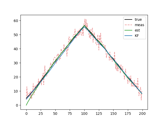
MHE diff: 0.5968899812607984
Measurements diff:  2.2559395317797053
KF diff:  0.6506733772967995
If the Guassian assumption about the noise were to change, updating the chance constraint can easily be done by changing the cclp_gauss call to call another cclp_risk_opt function.